Multiresponse Parameter Estimation: The α-Pinene Kinetics Case Study
A worked example of fitting a reaction-kinetics model to correlated, dependent measurements using the determinant criterion and rotated responses (Bates & Watts).
The problem
Classic weighted least squares assumes each measured response is independent of the others. But in many chemical kinetics experiments, several species are measured simultaneously from the same run, and their measurement errors are correlated — sometimes strongly so, because the responses are tied together by physical constraints like a mass balance.
The α-pinene pyrolysis dataset (originally due to Fuguitt & Hawkins, later analyzed by Box, Hunter, MacGregor & Erjavec in the 1970s, and used as a teaching example by Bates & Watts) is a good illustration. Purified α-pinene was heated, and the relative concentrations of α-pinene and three by-products — dipentene, allo-ocimene, and pyronene — plus a dimer were tracked at 8 time points. That’s 5 “responses” per run, governed by a linear kinetics model:
- α-pinene decays into dipentene and allo-ocimene
- allo-ocimene further decays into pyronene and the dimer, with a reverse path from dimer back to allo-ocimene
This gives a 5-parameter linear ODE system (rate constants θ₁ … θ₅, fit on a log scale so they stay positive).
Why you can’t just fit all 5 responses directly
Two things break the naive approach here:
- A mass balance. All five concentrations are percentages of the same starting material, so at every time point they must sum to (approximately) 100%. That’s a hard linear constraint on the data — not just a correlation.
- An imputed response. One of the five reported concentrations (pyronene) wasn’t actually measured independently in the original experiment — it was backed out from the others via the mass balance. So it carries no new information; including it in a naive least-squares fit just double-counts data you already have.
Both of these show up as near-zero singular values in the singular value decomposition of the centered data matrix — a standard diagnostic (Box, Hunter & MacGregor) for detecting linear dependencies in multiresponse data before you try to fit anything:
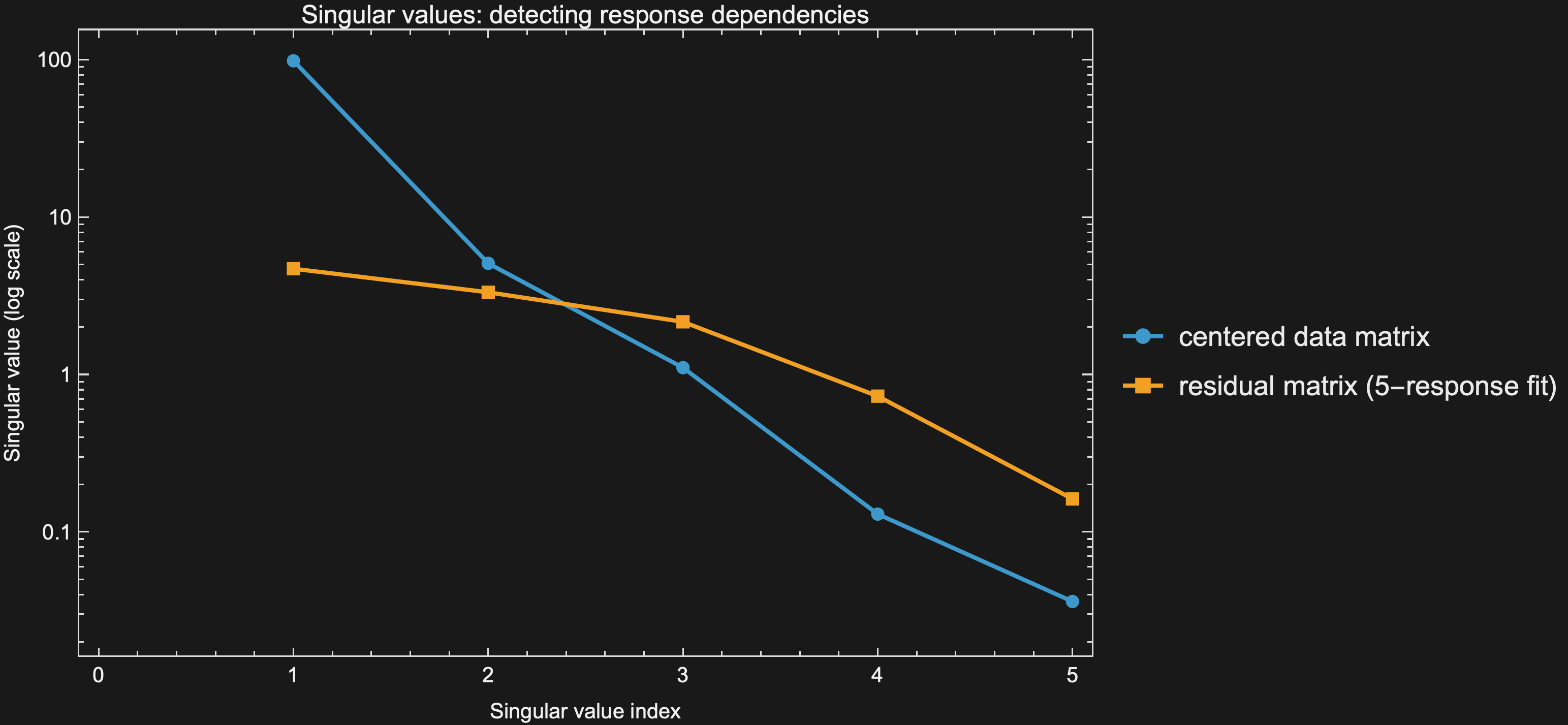
The two smallest singular values here are orders of magnitude below the largest, confirming two independent linear dependencies in the 5-response data — consistent with the mass balance and the imputed response.
The fix: rotate to independent responses
Rather than guessing which raw responses to drop, Bates & Watts describe a cleaner approach: build a small matrix encoding the known dependencies (the imputed-response direction and the all-ones mass-balance direction), and use a QR decomposition to find an orthonormal basis for everything orthogonal to those directions. Multiplying the data (and the model’s predictions) by that rotation matrix collapses the 5 correlated responses down to 3 independent rotated responses, with no loss of real information.
Fitting then proceeds by minimizing the determinant of the residual cross-product matrix for these 3 rotated responses — the standard multiresponse estimation criterion (Box & Draper). There’s a numerical wrinkle worth flagging: evaluating this criterion by literally forming the residual cross-product matrix and taking its determinant is numerically fragile, because forming that cross-product squares the condition number of the underlying residual matrix before you’ve even tried to take a determinant of it — exactly the kind of thing that erodes precision during an iterative search. Bates & Watts’ original computational device avoids this by evaluating the criterion through a QR decomposition of the residual matrix directly, never forming the cross-product at all: with Z = data.Bmat - fpred.Bmat and {q, r} = QRDecomposition[Z], the criterion is 2*Total[Log[Abs[Diagonal[r]]]], since |Zᵀ Z| = |R|² and the log of a squared diagonal product is just twice the sum of the log-magnitudes. That’s the approach used here, paired with Wolfram’s FindMinimum as the optimizer rather than their originally proposed Gauss–Newton iteration, which predates general-purpose optimizers being routine.
Results
Fitting the rotated 3-response problem gives rate-constant estimates (on a log scale, θᵢ = exp(φᵢ)) that match the published analysis closely:
| Path | φ (log-scale rate) | Rate constant θ (×10⁻⁵ min⁻¹) |
|---|---|---|
| α-pinene → dipentene | −9.73 | 5.94 |
| α-pinene → allo-ocimene | −10.47 | 2.86 |
| allo-ocimene → pyronene | −12.31 | 0.45 |
| allo-ocimene → dimer | −8.07 | 31.1 |
| dimer → allo-ocimene | −9.76 | 5.79 |
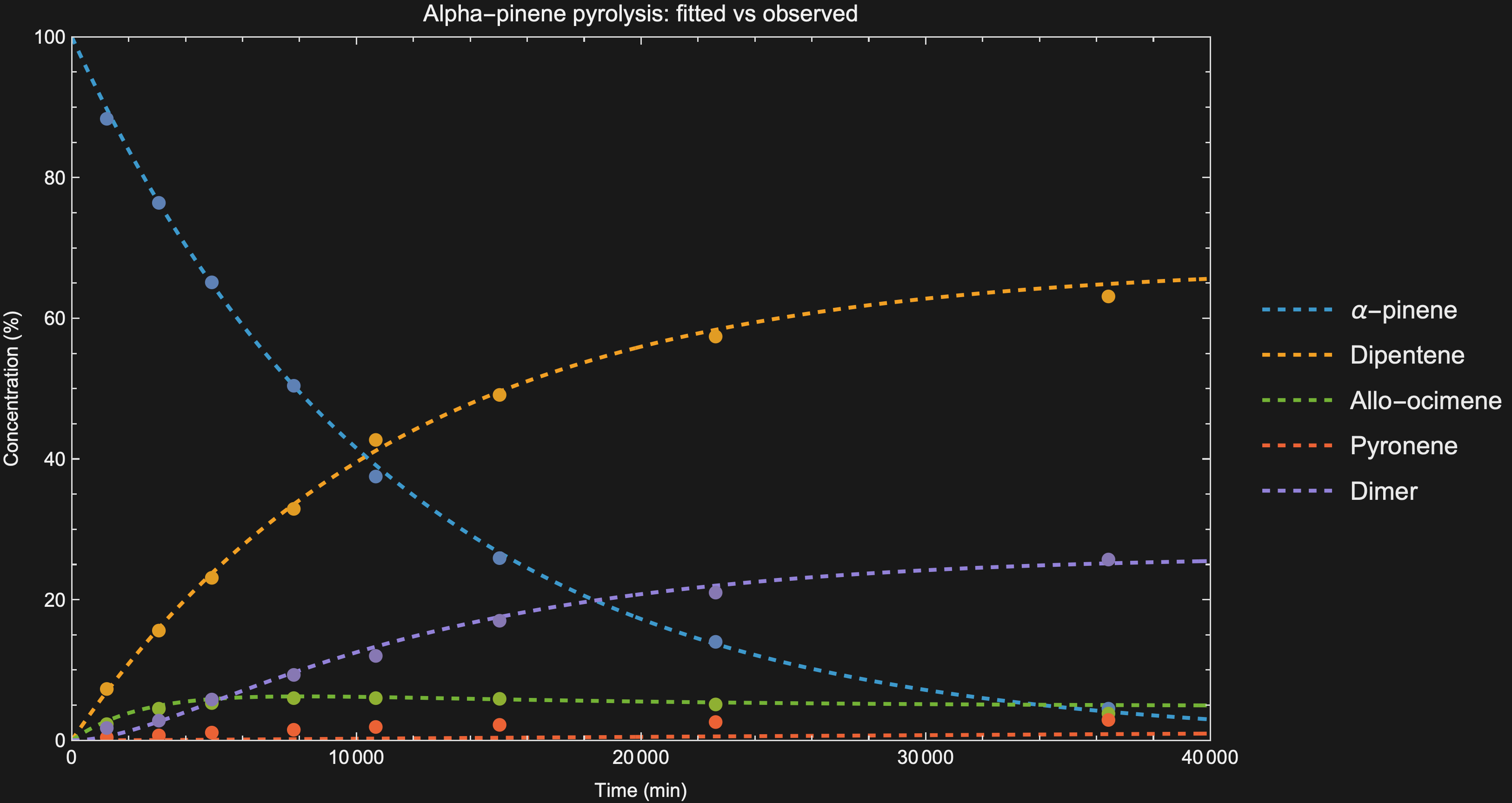
The fitted curves track the observed concentration profiles well across all 5 species (recall: the rotation is only used for fitting — once we have θ, we can simulate and plot all 5 original responses):
Model criticism
Two standard checks worth showing on the page:
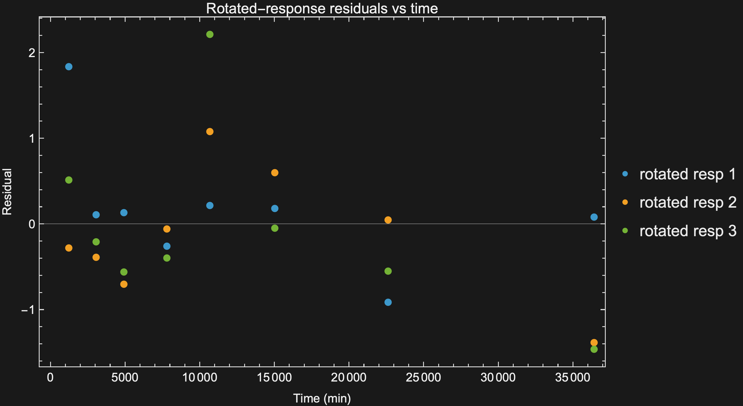
Residuals of the rotated responses, plotted against time, should look patternless if the kinetic model is adequate — no trend, no systematic sign pattern:
Which directions in parameter space are poorly identified. Rather than looking at each parameter’s standard error in isolation, it’s more informative to eigen-decompose the approximate parameter covariance matrix (from a Fisher-information-style approximation around the optimum) and look at its eigenvectors. Four of the five eigenvalues are small and comparable in size; the fifth is about 200× larger than the next-largest, and its eigenvector is almost entirely a single component — better than 99.9% of that direction’s length is the allo-ocimene → pyronene path (φ₃), with the other four parameters contributing almost nothing. That’s a much sharper diagnosis than “φ₃ has a large standard error”: the poorly-identified direction in parameter space isn’t some blend of several rate constants — it’s essentially pure φ₃, in isolation from everything else in the model.
A different lens on the same theme
The core question here — how many parameters (or how much of the data) can you responsibly use, given limited, correlated, or noisy measurements — shows up under a different name in Kimberley McAuley’s group’s work on model selection criteria. Eghtesadi, Wu & McAuley’s Development of a Model Selection Criterion for Accurate Model Predictions at Desired Operating Conditions (Ind. Eng. Chem. Res. 52, 12297–12308, 2013) tackles a related but distinct problem: rather than asking how to combine correlated responses (this page’s question), it asks how many parameters to estimate from a model when data are too sparse or correlated to estimate all of them reliably, using a mean-squared-error criterion that trades off bias against variance. Their group’s broader body of work leans heavily on weighted least squares as the workhorse estimation method, extending it (via error-in-variables models) rather than replacing it — a useful contrast to the determinant-criterion route taken here. I had the chance to meet Dr. McAuley at NASCRE-5, where this connection came up directly.
What this page deliberately leaves out
This page sticks to the estimation method itself (weighted least squares generalized to the determinant criterion, with the rotation trick for handling dependent responses) rather than getting into the fully Bayesian treatment of the same problem (posterior densities over Θ and Σ, Cholesky-based numerically stable likelihood evaluation, HPD regions). That’s a deeper rabbit hole that’s more appropriate for a follow-on technical note.
Want the Wolfram Language code behind this? It’s not proprietary — the method is straight out of Bates & Watts — but a few of the tricks in it (using SingularValueList to catch data dependencies before fitting anything, eigen-decomposing the parameter covariance to isolate a poorly-identified direction) aren’t things you see every day in a chemical engineering context. Get in touch and I’m happy to send it over.