Split-Plot Designs: The Corrosion Resistance Case Study
Why pretending a restricted-randomization experiment was fully randomized can mislead you — in either direction.
The setup
This is a classic teaching example from Box, Hunter & Hunter’s Statistics for Experimenters (Chapter 9): steel bars are coated with one of four coatings (C1–C4) and their corrosion resistance is measured after exposure. The coatings are baked on in a furnace at one of three temperatures (360°C, 370°C, 380°C), with 6 furnace heats total.
Here’s the catch: temperature is hard to change — you load a furnace, set it to one temperature, and bake everything in that batch together. Coating is easy to change — within a single furnace heat, you can randomize which of the 4 coated bars goes where. So each experiment isn’t fully randomized; it’s a split-plot design:
- Whole plots = the 6 furnace heats (temperature applied at this level, one temperature per heat)
- Subplots = the 4 coatings within each heat (randomized within a heat)
This kind of constrained randomization is everywhere in real industrial experiments — anything where one factor is expensive or slow to change and another isn’t. The statistical consequence is that there are two different error variances, not one: the heat-to-heat variance (how much whole plots differ from each other) and the within-heat variance (how much subplots differ from each other, after removing the heat’s own average). Temperature’s significance has to be judged against the first; coating’s significance has to be judged against the second.
What happens if you ignore this
The tempting shortcut is to throw everything into one linear model — temperature, coating, their interaction — and run a single F-test against one pooled residual. Doing that here:
| Source | df | F | Conclusion |
|---|---|---|---|
| Temperature | 2 | 10.2 | Looks significant |
| Coating | 3 | 1.1 | Looks non-significant |
That’s backwards from the truth. Pooling the two error strata into one blends a small, noisy sample of whole-plot variation with a much larger, cleaner sample of subplot variation, and the result can distort the picture in either direction depending on which stratum’s variance dominates — here it makes the hard-to-change factor look important and the easy-to-change factor look unimportant.
The correct split-plot decomposition
Splitting the analysis into its two proper strata:
| Whole Plots (Temperature) | df | SS | MS | F (p) |
|---|---|---|---|---|
| Temperature | 2 | 26,519 | 13,260 | 2.75 (p = 0.21) |
| Error (whole-plot) | 3 | 14,440 | 4,813 |
| Subplots (Coating) | df | SS | MS | F (p) |
|---|---|---|---|---|
| Coating | 3 | 4,289 | 1,430 | 11.48 (p = 0.002) |
| Temperature × Coating | 6 | 3,270 | 545 | 4.38 (p = 0.024) |
| Error (subplot) | 9 | 1,121 | 125 |
The conclusion flips entirely: temperature’s effect is not statistically significant at this sample size (p = 0.21) once judged against the right error term, while coating’s effect is clearly significant (p = 0.002) — the opposite of what the naive pooled analysis suggested.
The two error variances themselves are informative on their own: the whole-plot standard deviation (σ_W ≈ 34.2) is roughly 3× the subplot standard deviation (σ_S ≈ 11.2), meaning heat-to-heat variability genuinely swamps within-heat variability here — exactly what you’d expect from a hard-to-change factor with only 6 independent replicates behind it, versus an easy-to-change factor with 24.
Seeing it
The same story, visually — wide error bars on the whole-plot (temperature) means versus tight error bars on the subplot (coating) means, plotted at their own natural precision:
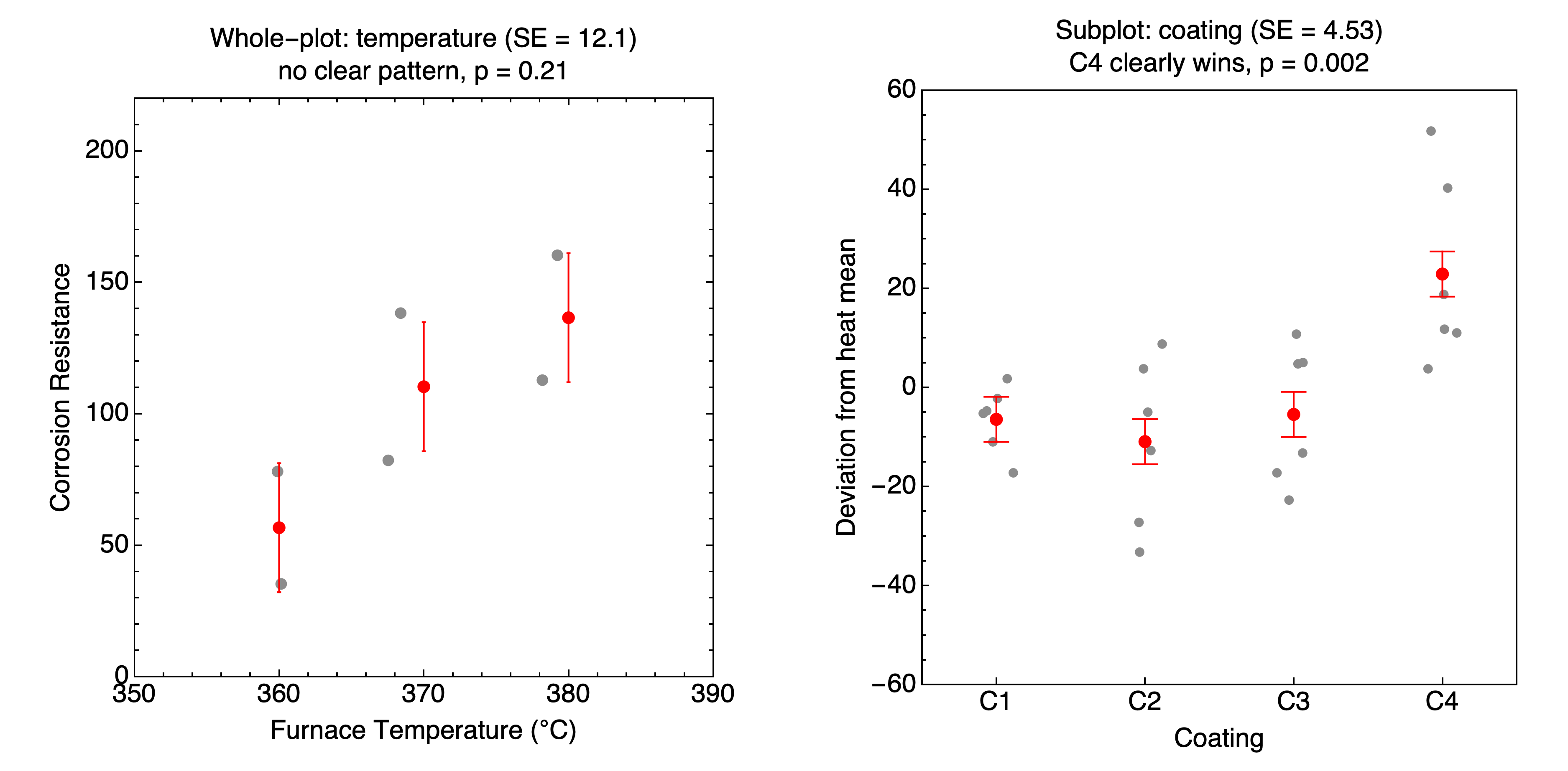
Coating C4 stands apart from the other three with a tight confidence interval; temperature’s three furnace levels overlap heavily once you account for how few independent heats back up that comparison.
The takeaway
Split-plot structure isn’t a nuisance to average away — it’s telling you something true about how the experiment was actually run, and the two error strata carry genuinely different amounts of information. Analyzing a split-plot design as though it were fully randomized doesn’t just cost you some statistical power; it can flip your conclusions about which factor actually matters.
Want the Wolfram Language code behind this? Get in touch and I’m happy to send over the script — the data, both the naive pooled analysis and the correct split-plot decomposition, the variance component estimates, and the summary plot.